“Predictions are hard, especially when it’s about the future” - Jacques Chirac
This is a hopeful blog: can we predict when civil wars are bound to occur ? If not, can we stop them ? Such events are profoundly destructive for the citizens of these countries, and their effects are now inevitably globalized. Predicting these conflicts early on presents a major challenge for policymakers in an effort for peace. By successfully doing so, the identification of potential causal mechanisms would unravel a world of possibilities when it comes to understanding and defusing these catastrophes.
Economical crisis, infant mortality, anocracy… When a civil war occurs in a country, retrospectively, one can say “of course this is happening, this country had so many major issues !”. But which issues in particular lead to civil wars ? Are some more influential than others ? Are there patterns triggering civil wars, some sort of evil secret sauce ? Can we avoid civil wars by predicting them, and acting before the irreparable ? That’s what we will try to find out.
What tools for prediction ?
This decade has seen the increasing use of machine learning techniques, deep learning in particular, in a broad range of areas. This renewed enthusiasm, in part triggered by the dramatic increase in data and computing power, has implications in the domain of the political sciences. In 2015, Muchlinski and colleagues released a study on the use of Random Forests, a machine learning technique well suited for the prediction of rare events: Comparing Random Forest with Logistic Regression for Predicting Class-Imbalanced Civil War Onset Data. One of their findings was that this machine learning technique could rival with classical statistical methods in predicting civil war onsets, and brought some new insights into the emergence of these conflicts by analyzing the predictive power of the variables used.
In a similar fashion, our study aims at pushing this comparative analysis further, in the realm of Artificial Neural Networks, and Multi Layer Perceptrons (MLPs) in particular. Since Random Forest algorithms are powerful at handling severe imbalance in the data to answer such questions, we wish to study if MLPs can do the same. If proven useful, MLPs could, for instance, enhance the prediction of rare events in conflict data by leveraging their high flexibility in input modality: be it temporal, linguistic or visual data. To motivate their use, we will focus on four different interrogations about these conflicts:
- Can we predict when they start ?
- Does this prediction change throughout modern history ?
- Can we find patterns in the predictors ?
- Can we predict when they end ?
This study presents some of the tools one can use when dealing with the prediction of rare events. We will go through the pipeline and analytical work needed to derive conclusions from predictive models, and raise some important questions as to the validity of these conclusions. But before diving into the core of this study, let us ask ourselves:
Civil what ?
Mark Gersovitz and Norma Kiger define a civil war as “a politically organized, large-scale, sustained, physically violent conflict that occurs within a country principally among large/numerically important groups of its inhabitants or citizens over the monopoly of physical force within the country”.
Between 1945 and 2000, no less than 116 civil wars occurred across the world. The map below shows the number of years a country has been in civil war. As we can see, Southern countries are the most impacted, in Asia, the Middle East, Eastern Africa and South America. Some countries, such as Colombia, have been in civil war for decades !
In this project, we were particularly interested in the onset of civil wars, which are presented in the map below:
Some countries, such as Nicaragua, India and Iraq have experienced up to 3 civil war onsets ! Looking at where these conflicts emerge, how some last while others come and go, one cannot help but wonder what role the geographical, economical and temporal patterns of these hotbeds play.
A good amount of literature about civil war causality exists, such as Fearon and Laitin (2003), Collier and Hoeffler (2004) and Hegre and Sambanis (2006). Those papers are based on civil war datasets: the one we based our research on is the dataset Amelia, a subset of Sambanis’s dataset, with features selected to be most relevant to predict civil war onset. We will leverage this data in order to answer the questions we raised.
Can we predict when they start ?
The best way to limit the impact of civil wars, is to prevent them. To do so, we can take a look at the past. By building systems able to predict the onset of these past events by relying on social, economical and geographical factors, we could hope to have forecasts for the future. By studying what factors do these systems rely on the most, we can get an insight into causality. But this task is not easy, and full of potential traps.
Our mission starts with the choice of tools. As explained earlier, we will use machine learning techniques to build models of the onset of these conflicts, in particular Random Forests and MLPs. The idea here is to predict on the data of a given year if a civil war onset happened by optimizing the models. Both of the models rely on a set of hyperparameters, of which the best combination is not known a-priori. In order to find the combination of hyperparameters which is most successful at predicting the onset of civil wars, we build a grid of possible values. Since evaluating the performance of these models on each combination of that grid would take too long, a random subset of these combinations are chosen, in the hope that the grid is well covered. This approach is called Random Search.
Based on our definition of performance, in this case the balanced accuracy (since the classes are imbalanced), the best combination for each model is chosen. We then plot the Receiver Operating Characteristic (ROC) curve, which is a measure of the performance of our model. Essentially what this curve tells us is how robust the model is to a change of decision threshold. Ideally, the model would be able to separate the classes well enough that the amount of false positives increases only for extreme values of the decision threshold. The Area Under the Curve (AUC) summarizes this effect, the larger the better:
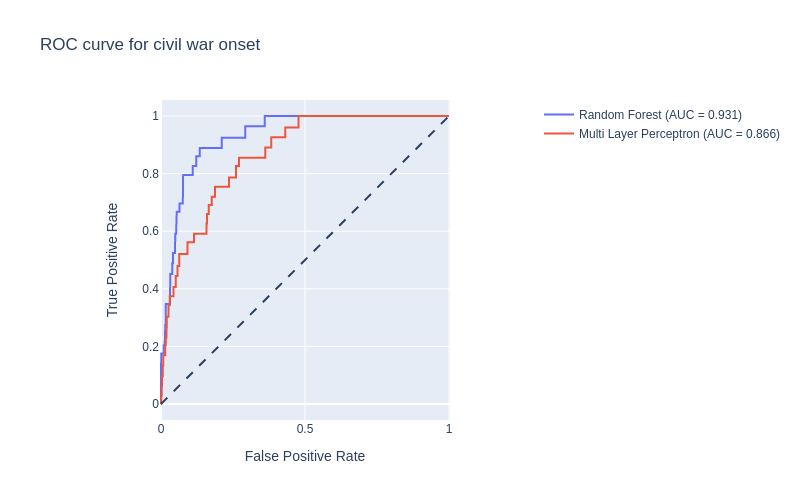
For both approaches the model is a good predictor of civil war onset, yielding high AUC scores. Since the ROC is evaluated on a subset of the data that the models have not been trained on, it shows that the systems are able to generalize well enough.
With good predictors at hand, we can start analyzing how they made their prediction. First, we dig into the synapses of the MLP by looking at the degree of activation of the neurons for each datapoint. Since the datapoints lie in a high-dimensional space equal to the number of neurons, reducing their dimensionality is crucial. For that, we use the probabilistic method t-SNE. To be prudent, we also apply the same treatment to the features and to the activations of an untrained MLP that we use as controls for our conclusions:
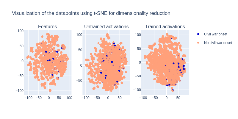
For the controls, it looks like the datapoints do not differentiate well from the civil war onsets. This could mean that there is no easy way to group the datapoints without further processing. For the trained MLP, the conclusion is a bit different. It looks like the datapoints of civil war onset tend to group towards the bottom-right, yet it is not very clear. This is still an insight into how the MLP processes the information in order to build nonlinear mappings from feature to prediction.
Now to the fun part: what feature do the models actually leverage ? To do so, we use a technique called Permutation Importance. The idea is that if the values of an unimportant feature for different datapoints are randomly shuffled, the performance of the model should not be too affected. Inversely, if the performance decreases significantly, the feature can be deemed important. The permutation importances are calculated on the test set so as to inform on the features that are important for generalization. In order to understand what all the acronyms of the features mean, you can refer to the replication material of the original paper. We will explain the meaning of the most important ones.
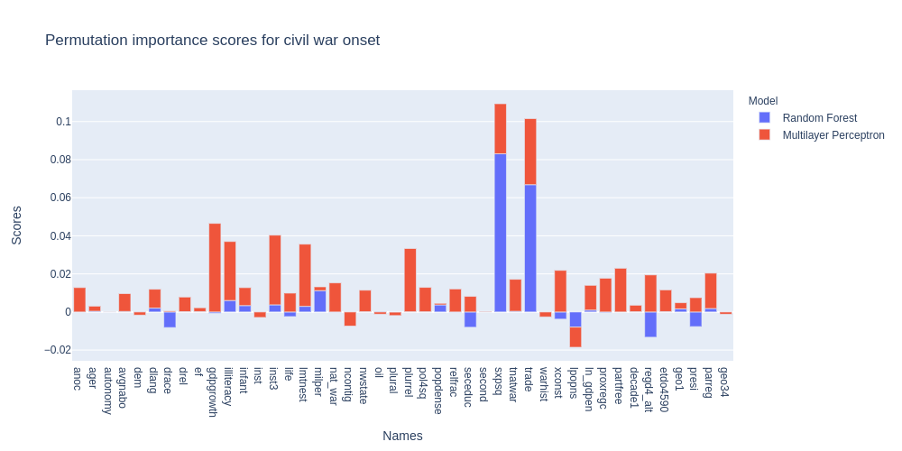
Two things come to mind: some features are very important for both models, and some features have different importance even if the two models have similar predicting power. This last points highlights that talking about causality when using machine learning techniques is risky, as different models can leverage differently the features for prediction. However, some features are clearly very important for both models, such as primary commodity exports/GDP squared (sxpsq), trade as percent of GDP (trade), autonomous regions (autonomy), rough terrain (lmtnest), percentage of illiteracy (illiteracy), and military power (milper). This analysis corroborates some of the results of the original paper with the new models. However, some features such as the GDP growth (gdpgrowth) show very little predictive power on the test set for Random Forest, which goes against what the original paper shows.
To verify these results, we will inspect some features on a world map. Let’s look at an economical factor, the primary commodity exports/GDP squared, during an onset or not:
We observe than indeed, countries experiencing a civil war onset have a noteworthy decrease in primary commodity exports/GDP. Peru for instance, has seen, on average, a drop from 0.05 to 0.006, nearly an order of magnitude difference.
Now, let’s inspect a social factor, namely the percentage of illiteracy:
Similarly, we see that states experiencing a civil war onset have higher rates of illiteracy. One staggering example is that of Afghanistan, where illiteracy increases from 34% to 83% on average.
Does this prediction change throughout modern history ?
Now we know that we can predict quite accurately when a civil war onset would occur, and we also found the important indicators to look at for the prediction. With this, we could prevent ourselves from having any civil war in the future, right ?
It is probably a bit more complicated than that. The first thing that comes to mind is that the reasons for civil war could change over time. In this part we will now try to tackle this question. Our first approach will be to train the models we already used before, a Random Forest classifier, and a MLP on data from different periods. Then we will analyze the feature importances on every period. To get the data from different periods, we separated the dataset into overlapping bins of 15 years periods, with intervals of 5 years. So, we made separate datasets with the data of the years 1945 to 1960, 1950 to 1965, 1955 to 1970 and so on. This gives us 9 bins of data, with a number of samples per bin varying from 1285 to 2596.
We will have to be careful about something already: by separating the data into bins, we reduced the number of samples for each model to train on. With the class imbalance, this could become a challenge. So for training those models, some other parameters were chosen by hand for the randomized grid search. The parameters were chosen mainly to prevent overfitting to singular civil war events since the number of civil war events is reduced in the bins, and therefore they have more singular characteristics. For this the number of parameters for each model was decreased (by adjusting the different parameters). After hand-tuning of those parameters, the models were trained on the separate data bins, with 20 iterations of the randomized grid search. The ROC curves for the trained models for each period are shown in the figure below.
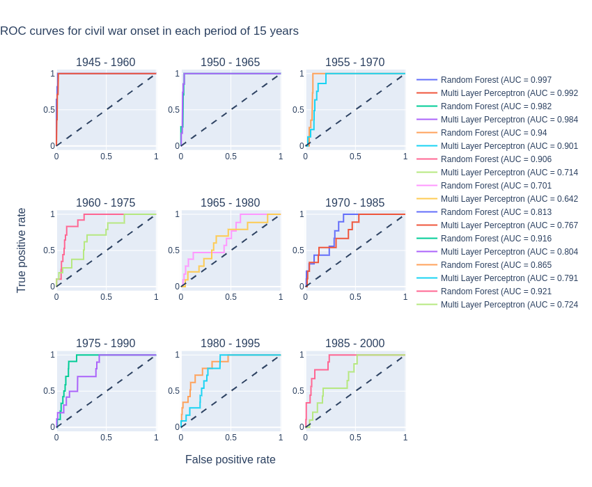
Let us analyze the performances of the models. For the first three periods, the performance is very good, we have areas under the curve over 0.9 for both models. The performance of the models on the 7th period and the 8th are quite good, with areas under the curve around and over 0.8. However, for the other periods, the neural network seems to be less performant, and for some of them, also the Random Forest is not performant. Generally, the Random Forest model does a better job on all the periods. The periods where the models are less performant, especially 1965 to 1980 and 1970 to 1985, could have a really small proportion of civil war onsets or the civil war onsets in these periods could have very different features, and are therefore difficult to predict. We will have to be careful about the analysis of the feature importances in those periods, since the models are poor predictors.
Now we will analyze the important features of each period. The scale of importance is logged in order to see all the importances scores, since some are orders of magnitude higher than the others. The following interactive plot shows the feature importances for each feature for each period. The slider changes the period visualized. It is important to note that since the importance scale is logged, the negative values do not appear.
We can see that the most important features change significantly from period to period. In the first period, it seems that only trade, the trade as percent of GDP, seems to have an importance for civil war onsets. seceduc, the percent of population with secondary education, has a slight importance. On the second period, other features play a role in the prediction: illiteracy, the illiteracy rate, is really important, as well as sxpsq, the primary commodity exports squared and infant, the infantile mortality rate. However, all these features found as important, only have an importance for the MLP. Therefore, doubts can be raised on their validity. In the following period, from 1955 to 1970, the most important features are the illiteracy rate, with a huge permutation importance of 0.5. The other important features are primary commodity exports squared, trade as percent of GDP and infantile mortality rate, with the 2 models agreeing on their importance. In the period of 1960 to 1975, only the Random Forest model seems to find important features. Here again the same features as before have an importance for civil war prediction. However, the illiteracy rate and infantile mortality rate have a 5 to 10 times decrease in importance between the previous period and this one. We start to see a change in important features. In the period of 1965 to 1980, the feature gdpgrowth, the GDP growth, seems to gain in importance for both models. The nat_war feature, indicating if neighbors are at war, seems to have an importance for the MLP. However, since the performance of this model is bad on this period, this is not very reliable. Actually, in this period, the Random Forest predictor also shows bad performance. In the following period, the predictors also have a poor performance, so this analysis should be taken with precaution also. However, the features inst3, the political instability index and gdpgrowth seem to have an importance for the MLP. For the Random Forest model, the illiteracy rate is still important in this period. In the period of 1975 to 1990, the trade is still important, and new features arise as important. life, the life expectancy, as well as dlang, the linguistic fractionalization index, show a slight importance. For the MLP, again less reliable, the secondary education, the governmental institution and the neighbors SIP score, play a role in civil war. In the period of 1980 to 1995, trade and primary commodity exports seem to be important for both models. For the Random Forest model, milper the military manpower is of importance. For the MLP, popdense, the population density and pol4sq, Polity 4 squared are valuable. However, here again the predictors are not perfect. In the last period, military manpower shows a great importance for both models, as well as GDP growth and illiteracy rate, with a lower importance.
This was interesting. However, we saw that the models sometimes disagree on the important features, or show low importances. Generally, when the models disagree, doubts can be raised. We also saw in some periods very few inputs from one or the other model. Actually, it is because in these periods, the permutation importances are negative, as we can see on a linear scale of importance in the following figure.
In the periods where the predictors are poor performers, a lot of feature importances become negative. This is indicating that the model and the feature importances on those periods are rather unreliable.
With this analysis, even if in some periods, the important features found are not robust, we saw that there are some features which stay important along all the analysis, though in varying importance, and others which arise in specific periods. This is due to specific civil wars depending on certain aspects. We can also see that the causes for civil wars still vary along the years, and while some features are not important for civil war onset prediction, others can have an importance in a period and not in another. This raises the question of the possibility and the validity of making models for the prediction of civil wars.
Can we find patterns in the predictors ?
An issue we can find in the previous analysis is that we were trying to find feature importances on fixed length of periods. This is not how it really works. It is rather that some indicators become more important in an undefined period of time, until they do not anymore. This is why in this part, we will use unsupervised learning to find some patterns in the features of civil war onsets, and then see if time is a separator between these found patterns. For this analysis, we will use clustering.
For this part, we have to concentrate on the civil war onsets events. Therefore our data is reduced to 116 samples. We will have to choose meaningful features to do the clustering on the features selected are chosen among the ones who were the most likely to set civil war in the previous analysis… Since the Random Forest models were generally better, we will take all the features which have a permutation importance higher than some threshold for the Random Forest model. We will add to this the top features of the MLP models which were not top features in the Random Forest model to complete to 20 features. Eventually, the selected features are the illiteracy rate, the infantile mortality rate, the primary commodity exports squared, the trade as percent of GDP, the GDP growth, the mountainous terrain, the population density, the linguistic fractionalization, the life expectancy, the the military manpower, the population logged, the GDP per capita, the median regional polity, a democracy dummy variable, executive constraints, secondary education, the neighbors average SIP score, the governmental institution, the political instability and the regulation of participation. These variables all sound meaningful !
Since the data of the features is on different scales, we will normalize the data. However, we have some binary data, which we will not normalize, in order to keep the information of separation between the 2 classes. Therefore we consider that for binary data, the distance between the 2 classes is maximal. Then, we have to reduce the dimensionality to get a better clustering, using principal component analysis. By doing so, we keep 90% of the explained variance in the data, reducing the number of dimensions to 12.
In order to classify the data, we have tried several clustering algorithms, which are OPTICS and K-Means. OPTICS is a variation of DBSCAN that chooses the epsilon parameter automatically. This method iss interesting because of its small number of hyperparameters and ability to cluster non globular clusters, which could be of importance here if multiple civil war onsets are due to only one feature. Another interesting capability of this method is to define outliers. This could reveal useful in our analysis since some civil war onsets could have totally different causes than some other groups. For this method, we have to firstly choose an appropriate distance metric. After looking at metrics for high dimensional data, we chose correlation as our metric since it yielded good results. Then, the parameter of minimum samples to construct a cluster has to be chosen. For this, we will do a parameter search.
To compare both methods and to choose the hyperparameters for each method, we use the silhouette score. To quote Wikipedia, the silhouette value is a measure of how similar an object is to its own cluster (cohesion) compared to other clusters (separation). The silhouette ranges from −1 to +1, where a high value indicates that the object is well matched to its own cluster and poorly matched to neighboring clusters… For the evaluation of the OPTICS algorithm, we also plotted the number of outliers: we do not want too much outliers, or the clustering has no use.
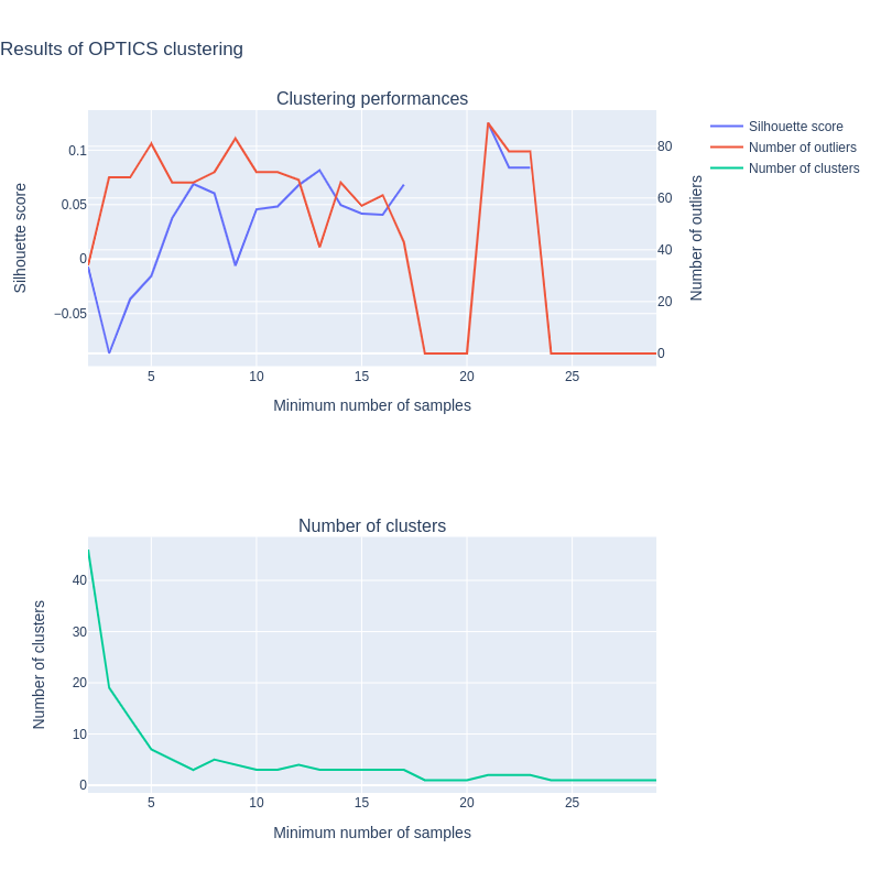
Firstly, we see that the clustering is not very good, the highest silhouette scores are around 0.1, and the number of outliers varies from 40 to 80 for acceptable silhouette scores. On a dataset of 116 samples, this is too much outliers. The high number of outliers also indicates that the data is not easily separable into clusters. The bad clustering is also due to our small number of samples, where it is hard to find patterns. However, if we have to choose a minimum number of samples, 13 seems to correspond to a high silhouette score with a smaller number of outliers.
So the next method in line is K-Means. For K-Means, we took the default L2 distance metric. We have to choose the number of clusters for this method. For this again, we use the silhouette score, and we also use the sum of squared errors (SSE), evaluating the distance of each point to its cluster center, and summing over all points and all clusters. The smaller the SSE, the better. However, the SSE is the smallest with the number of clusters equal to the number of points, which is not a good clustering. Therefore, the method is to search for the “elbow” in the descending SSE curve, where the curves becomes flatter.
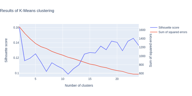
Here the results seem better, with silhouette scores of 0.12-0.15. So we decided to use K-Means as our final clustering algorithm.
Concerning the number of clusters, we have found slightly changing results as we ran the notebook different times. This happens because we have a small dataset, so there model changes a lot. Moreover, K-Means is initialisation-variant, which increases variations between iterations. However, the Python K-Means method implements iterations of the clustering to find the best one. Still, both models allow us to say that the number of clusters is variant between 13 and 15. Still, we can see the “elbow” at 15 clusters on the sum of squared errors, It also corresponds to an acceptable silhouette score. Therefore we will choose 15 as the number of clusters for the final clustering. As we saw, the clustering is not perfect and we should be doubtful about this result.
So, are there tangible results ? Can we really find “evil secret sauces” (e.g patterns) of features to trigger civil war ? To answer this question, we have two reading grids : the clustering of the whole dataset, and the evolution of the cluster`s relative importance across time.
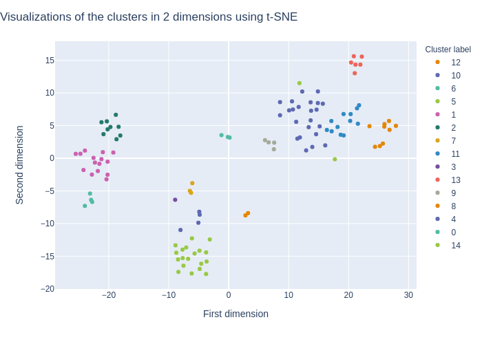
We get a good overview of our clustered dataset by using t-SNE. We can see by looking at the following graph that the clustering result is mixed. We can see that the points are consistent with the clustering, but the clusters do not appear clearly separated on the graph. This could also be due to the fact that t-SNE does not use the same methods as K-Means for clustering and this visualization is just an indication of the results.
The next big question, our initial interrogation, is the distribution of clusters across time. For this we plotted the clusters in violin pots, with respect to the time of the civil war onset.
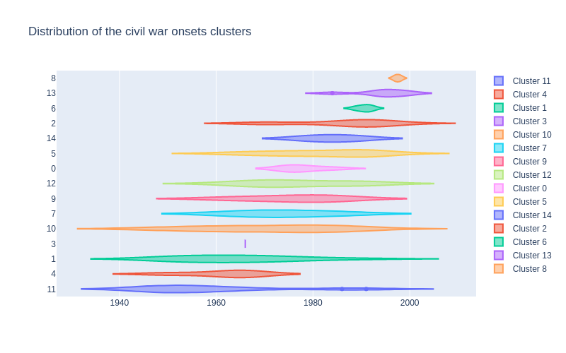
We can see that the clusters actually range over quite some periods. For some clusters, they are quite narrow in the time range. This would indeed mean that we found some civil war onsets which had similar causes due to their period of onset. However, all clusters are not clearly timely separated. This could be due to various things. Firstly, we found similar causes in the civil war onsets, and these causes could spread over a wide range of years, or these causes could have no relation with temporality. Therefore, the clusters would encompass some causes inherent to civil wars over all years. This would be very interesting, since these causes could be indicators for future civil wars. It could also be that the data is not easily clusterable, and the clusters found are not very reliable.
We can consider the result of this clustering part as mixed: the dataset we use is small, especially compared to its dimensionality, which makes clustering complicated. The silhouette score is not very high. However, our initial question was if we would be able to find clusters and dependencies, and the silhouette score was not expected to be very high. Still, the violin plot shows some clusters that seem to be short and thick enough to be considered as “typical of their epoch”.
Can we predict when they end ?
We are starting to get insights into civil war onsets. But say our system fails to predict a particular civil war onset, and that it is too late for policymakers to act. Is there any way that we can stop the civil war early on ? To answer that, we employ a similar approach to the prediction of civil war onsets. Namely, we will try to predict when a civil war ends. To do so, we will modify our dataset in order to add a new feature: the end of a war. For this feature, a positive means that the civil war ended that year, and a negative means that the war is still active. For that task, we have to discard a large portion of the data and keep only the data corresponding to countries at war or countries that have just entered peace: our predictor will try to differentiate the two.
After performing our random search and found good candidates for our models, we plot the ROC curves:
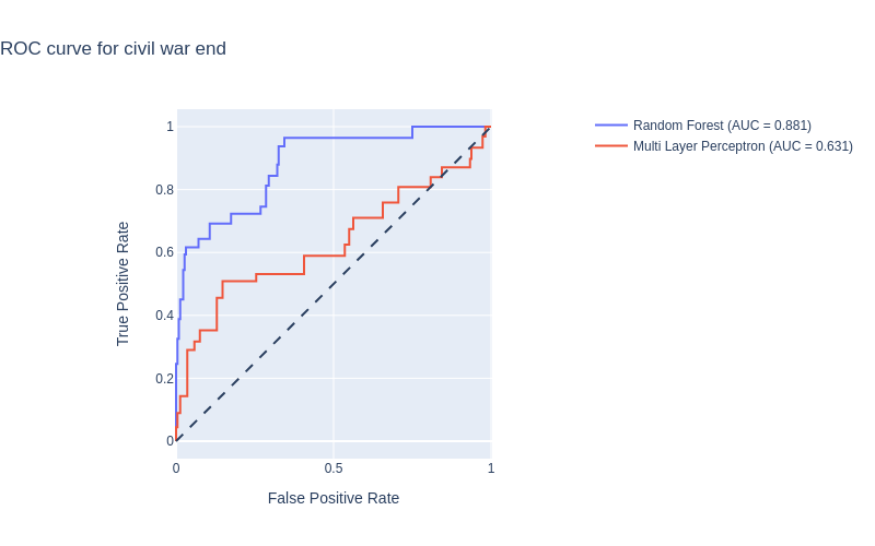
Surprisingly, despite the low amount of data, the Random Forest model performs well. However, similarly to what was mentioned above, the MLP seems to be performing much worse than the Random Forest. Still, the model is better than chance. It is probable that the very low amount of data and the high class imbalance is causing these results. Let us take a look at the MLP and plot the activations to better understand what is happening:
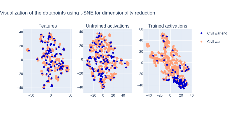
We see that for the trained MLP, the activations cluster well compared to the controls. However, we can see that the datapoints still overlap, causing the performance of the model to decrease. Even if the MLP managed to extract a nonlinear mapping from the data, it might be that the amount of data was too scarce for the MLP to make that mapping more robust.
Since our Random Forest model has high predictive power, can expect to learn something from the permutation importance scores:
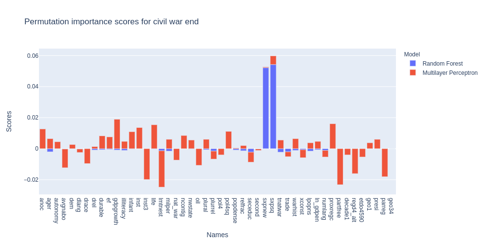
Before overinterpreting the importance scores of the MLP, let’s not forget that the MLP had low predictive power. Still, we see that the permutation importance is high for economical factors: primary commodity exports/GDP (sxpnew) and it’s squared variant (sxpsq). Note that here, the feature sxpnew has been brought back to life: the reason being that these economical factors are the best predictors for the end of a civil war. Are exports stopping the civil war ? Let’s not jump to conclusions. In fact, because of how the dataset is made (in bins of one year), it is difficult to know what is the order of causality here: is the ending of the war due to large numbers of primary commodity exports/GDP, boosting the economy and assuaging the minds leading to the end of the conflict, or are the good numbers a result of the end of the war, since the economy can now thrive again. We cannot know this from this dataset, but looking at smaller time bins (such as months) would help us in understanding the ending of conflicts better.
It is clear here that primary commodity exports/GDP are on the rise in years where the civil war ends. For instance, Mali shows an increase on average from 0.01 to 0.05. Is it due to the end of the civil war, or has this triggered the end of the civil war ? Good question. It’s your turn now, assemble some data, and let us know !